R Notebooks and Reproducibility

Introduction

One of the key benefits of using R is that all of the actions associated with your analysis can be executed through computer code that you’ll be writing. This is great for three reasons:

1. Writing code creates a record of every step you’ve taken, so when you turn off the computer (or step away from the analysis for a few days), you can very easily re-trace your steps. Journalists also repeat some of the same steps across analyses, and they can thus easily copy and paste code to get their work done faster. (This also applies when you receive an updated version of a dataset — all of your analyses can be quickly replicated!)

2. It is easy to share your R code, which in turn increases journalistic transparency, which has been linked to trust in journalism. This enables others to dissect how journalists did something and even replicate their analyses. (Some organizations, like FiveThirtyEight and The New York Times will sometimes post the data and code behind their projects to platforms like GitHub in order to be more transparent.) It also enables journalists to learn from each other and build on each others’ work.

3. It makes it easy to clean and transform data without editing the original data files. It is a best practice to always keep an original (untouched) copy of the data that you can come back to.

This is a stark contrast to point-and-click tools like most spreadsheet software, which don’t keep detailed records of user actions. For example, if you edit the value in a cell, you will just see the new value (there’s no history of changes to that cell), and it is not always easy to “track changes” when it comes to spreadsheets. Put another way, a key benefit of using R in journalism is that it enables us to create reproducible journalism.

R Notebooks

It is very helpful to produce R Notebooks when using R to analyze data. R Notebooks allow you to present a human-readable write-up alongside your code (and the results of the code). That, in turn, can help you organize your code and thus achieve two additional objectives:

1. You can use your notebook to describe, on conceptual and logical levels, what you are aiming to do and follow it up with the code used to accomplish that objective. (This means that you’re not just seeing the final code but also getting some insight into how the journalist was thinking about the problem.)

2. Your code becomes even more reproducible because R Notebooks help to contain everything within a neatly organized package. When you knit your notebook for sharing, it performs your analysis from scratch and will produce an error if you omitted a step along the way. This increases your confidence that you’re sharing everything you did when you share your notebook files.

For these reasons, I strongly recommend that you get used to doing all of your analyses in R Notebooks from the very beginning.

Creating an R Notebook

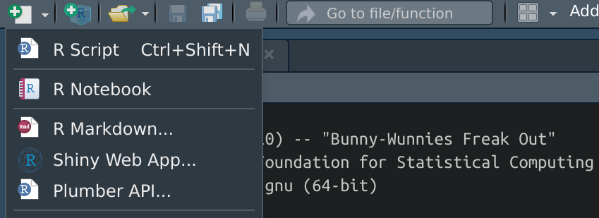
To create an R Notebook, simply load RStudio, click on File, New File, and R Notebook. Alternatively, you can just click on the icon with a white paper and a green plus sign that is below the File menu and select R Notebook there:

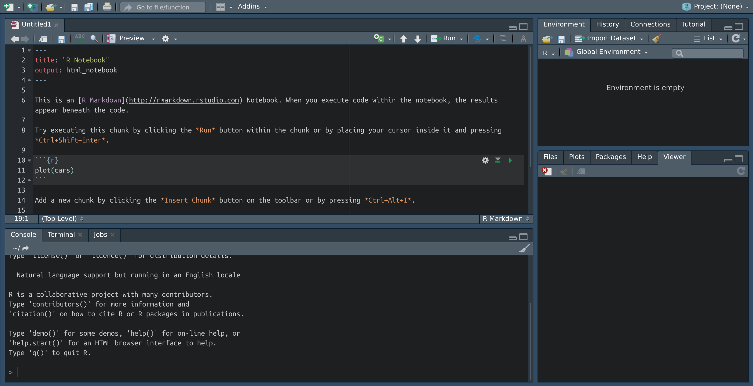
You should see a new pane open in the top left portion of the screen (we call this the Source pane) that looks like this:

Notebook Heading

At the start of a the default R Notebook, you’ll see the following:

---
title: "R Notebook"
output: html_notebook
---

Everything appearing between the three dashes at the top of the file is treated as heading/metadata information (we call this the YAML) header). This block of text allows you to fine-tune what our notebook will look like when we are ready to publish it via a process we call knitting.

You can adjust the settings by specifying different key:value pairs. For example, the title key refers to the title of the notebook, which we can set via the string "R Notebook". The output refers to the object that will be produced when we knit the notebook. We can also add certain keys like author and date to specify those details. Here is a full list of YAML header options that we can use in our R Notebook.

Here are some settings I like to use in my YAML header:

---
title: "Learning Challenge #X"
author: "Rodrigo Zamith"
output:
  html_document:
    code_folding: show
    df_print: paged
    theme: spacelab
    highlight: pygment
---

Notebook Text and Styling

Below the YAML header, we see the contents of our notebook. There are three main types of content: (1) Text, (2) Code, and (3) Output.

You can think of Text content as the notes you want to leave for yourself (or would like others to easily read). For example, you may want use Text to explain what your notebook pertains to (e.g., a story on climate change), explain where you got the data from, or why you decided to transform the data in a particular way.

We have many options for styling our Text content by using R Markdown syntax. For example, you can surround text with backticks (`, which are also called grave accent marks) to delineate code (like this: `code`). You can use a single asterisk (*) to specify italics (*italics*) and two asterisks to specify bolding (**bolding**).

To create a heading, use pound signs (#) at the start of a new line (e.g., # Heading 1). You can create lower-order headings by adding more pound signs (e.g., ## Heading 2), all the way up to the sixth level (e.g., ###### Heading 6). It is very helpful to use headings to convey the hierarchy of your document.

You can also create links by using the following syntax: [link text](URL).

There are many other styling options you can use by referencing the R Markdown Guide.

Writing and Executing Code

The second main type of content is Code. While Text covers instructions we leave for ourselves and other human beings, Code covers the instructions we are giving to machines.

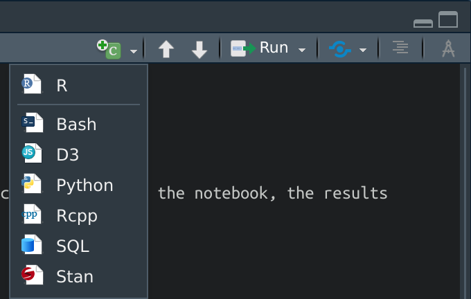
Code should be placed within Code Chunks in an R notebook. These are spaces reserved exclusively for code. To insert a code chunk in your Notebook, move your cursor to where you want to insert the chunk, click on the green “C” icon with a plus sign next to it that appears in the top-right corner of your Source pane, and select “R”:

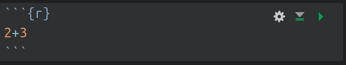
After you do that, you should see a new chunk appear that looks like this:

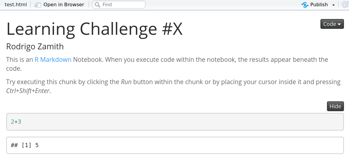
The three grave accent marks (`) are what designate something as a code chunk, and the {r} designates it as a chunk for R code.

The space in the middle is where we would enter the code we want to execute. For example, let’s say that we want to perform a simple arithmetic operation where we add two and three. We would organize our chunk like this:

To actually execute the code, we have two options:

1. The first option is to execute all of the code in that chunk. To do that, simply click on the green arrow in the top-right corner of the chunk.

2. The second option is to execute some of the code in that chunk. You can do that by simply highlighting the portion of the code you want to execute and pressing pressing Ctrl+Enter. If you don’t select anything, that key combination will execute all of the code appearing in the line where your cursor is sitting.

When you execute the code, the Output (result of the code) will appear immediately below the chunk:

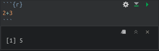
Behold, the result of our simple arithmetic operation is 5!

Knitting Your Notebook

While we can execute code chunks within our editor and see the results in real time, we will want to eventually use the knit functionality in RStudio to produce a properly formatted, nice-looking document that we can share with others. (And, of course, to submit assignments for your classes.)

To knit your notebook, go to File and select Knit Document. If you have not yet saved your R Notebook, it will ask you to save that first. Then, a new window should pop up that will show you a (hopefully) pretty document.

Do note that when you knit an R Notebook file, it will execute everything in your Notebook from scratch. Thus, if you’ve executed any code outside of the Notebook (e.g., loaded a package or a dataset using RStudio’s prompts), it won’t be considered part of the document — and will likely result in error messages. So make sure you work exclusively within the Notebook (and not the Console) for best results.

In most cases, everything you need to share your notebook with others (including any images, graphs, etc.) will be self-contained in the resulting HTML file. Thus, you can just e-mail that file to someone, publish it on R-Pubs, or submit it via Moodle and they will be able to see your Text, Code, and Output.