Describing Central Tendencies and Spread

Introduction

There are two main types of statistics that you should be aware of: descriptive statistics and inferential statistics.

Simply put, descriptive statistics just describe features of the data that you have on hand. A great deal of the data journalism done by mainstream news organizations relies mostly on descriptive statistics.

In contrast, inferential statistics seek to infer from the dataset on hand and generalize the information to a broader population. They allow the analyst to do things like project the future likelihood of something happening, to extend the insight gleaned from a small group to a larger one, and to simultaneously test the effects of each variable in a group on a dependent variable. You are more likely to see the use of inferential statistics in more niche sites that report on scientific studies (e.g., STAT) or data journalism outlets that employ statisticians (e.g., FiveThirtyEight).

Inferential Statistics

Inferential statistics are much more complicated to use than descriptive statistics because they require an understanding of the assumptions that underlie different statistical tests.

For example, a common inferential statistical test like a linear regression requires that the modeled data have residuals that are normally distributed, residuals that have constant variance, and values that are independent — in addition to adopting the assumption that any potential relationship is linear in nature. Put another way, you can run a linear regression on any dataset, but the results will be meaningless (if not misleading) if those assumptions are not checked and satisfied.

It is simply not possible for me to cover a sufficient range of topics in statistics within this book in order to promote the use of inferential statistical analyses. In fact, I strongly recommend against trying to perform any inferential analyses before taking a proper statistics course. Put simply, I would rather you not use inferential statistics than to use them poorly.

More broadly, it is important that you understand that if you do not understand a statistical test, do not use it in your analyses and reporting. If that analysis has been run in an improper manner, you will likely end up misinforming your audience — and that can have serious consequences to public understanding of a phenomenon in light of the mythology connected to advanced statistics (i.e., that it is a superior and more trustworthy way of ascertaining reality).

Descriptive Statistics

When it comes to descriptive statistics, there are two particularly useful sets of measures for data journalists: central tendency and spread.

Measures of Central Tendency

Measures of central tendency are useful for getting a sense of what is “normal” or “average” in the data. These measures include the mean, median, and mode of the data.

Mean

The mean is the most popular and well-known measure of central tendency, and it is often (incorrectly) referred to as the “average.” (In fact, the Google Sheets formula for measuring the mean is =AVERAGE().) You can calculate the mean by simply taking the sum of a sequence of values (numbers) and divide it by the count of those values. The result, or mean, may not actually be a value in your sequence and that’s perfectly okay.

For example, if I had 5 people that weighed 110 pounds, 120 pounds, 160 pounds, 140 pounds, and 210 pounds, the mean weight for those individuals would be 148 pounds ((110+120+160+140+210)/5 = 148).

Median

The median refers to the middle value in a sequence of values after it has been ordered by magnitude. Here, you will just want to take your sequence of numbers and reorganize it so that it goes from the minimum value to the maximum value, and work your way to the middle by striking the endpoints.

For example, with the aforementioned data, I would reorder those weights so it would be: 110, 120, 140, 160, and 210. First, I’d strike off 110 and 210. Then, I’d strike off 120 and 160. This would leave me with 140, which is the median weight in my data.

If you have an odd number of values in your sequence, the median will always be a value present in your sequence. If you have an even number of values, you would take the mean of your two middle values, which may result in a value that is not in your data.

Mode

The mode refers to the most frequent value in a sequence. The mode is rarely ever used in data journalism, but it can be useful for identifying a bimodal distribution (a distribution that has two peaks).

For example, you might have data covering the height of high school basketball players and find yourself staring at a bimodal distribution. You might find this interesting and explore the distribution of heights more closely, eventually finding that you actually have two distinct groups, with males typically being taller than females. Thus, simply reporting on an “average” height for the whole dataset might be far less informative than reporting it for two different groups.

Choosing a Measure of Central Tendency

Any of these three measures — the mean, median, and mode — can represent the “average” case in your data. So, which one should you choose?

The answer depends on the context.

For example, let’s say we have data on my bar tabs over the past month: $7, $8, $8, $10, $7, $20, and $275. The mean for my bar tabs would be $47.86. If I’m drinking at my local, cheap-o college bar, that might suggest it’s time for an intervention! The median tab, however, would be just $10. That is far more reasonable and representative of how much I typically spend at an outing to the local bar. (Moderation is cool!)

The most useful shortcut to help a data journalist decide which measure of central tendency to use is to see if there are any outliers (extreme values) in the data. If there is an outlier (as is the case for my $275 tab, which perhaps as I bought a round for the whole bar while celebrating some good news), then the median is the best option because it reduces the influence of that outlier. If there are no outliers, either measure should be okay — with the mean typically being used most often due to its preexisting association with the idea of an “average.”

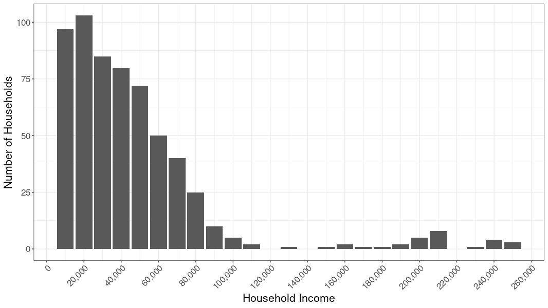
Similarly, let’s say we have an asymmetric distribution of numbers, as with a dataset covering income in a de facto segregated community, wherein we have a lot of folks clustered on the left end of the distribution (majority low-income people) and a long tail of wealthy people (minority of people spread out on the right end). This is called skew, and the key thing to look for is a tail in either direction.

When you have a highly skewed distribution, the median value is usually more informative than the mean (because the values in the tail end are not as influential). When the skew is minimal, either the median or the mean is acceptable. When the distribution is normal (the left side of the distribution is a mirror image of its right side), the median and mean will be the same value.

Additionally, if you have a variable that is nominal — meaning its values consist of names and thus have no numerical value, such as Honda and Subaru — then your only measure of central tendency is the mode (i.e., how often each label comes up).

Measures of Spread

Measures of spread are useful for getting a sense of how the data are distributed and how much variability there is in the data. These measures include the range and quartiles, and standard deviation.

Range

The range is the most common measure of spread in a sequence of numbers. It simply expresses the difference between the smallest and largest values in a set of data and serves as an indication of dispersion.

The simplest way to calculate the range is to order the values from smallest to largest and pick the values on the two ends. In the earlier example of people weighing 110 pounds, 120 pounds, 140 pounds, 160 pounds, and 210 pounds, the range would be from 110 pounds to 210 pounds.

Quartiles

Quartiles refer to the values of subdivisions of a ranked set of data. For example, the first quartile would refer to the value in the 25th percentile, the second quartile in the 50th percentile, and the third quartile in the 75th percentile.

A simple way to calculate this is to first take the median of a sequence and divide the ordered data into two halves. The median of the lower half represents the first quartile. The median of the entire sequence represents the second quartile. The median of the upper half represents the third quartile. The minimum and maximum values round out the 0th and 100th percentile, respectively.

Quartiles are a common instance of quantiles, which are the cutpoints for dividing the range of a probability distribution into contiguous intervals with equal probabilities. So, it is possible to calculate the values at other percentiles as well.

Standard Deviation

The standard deviation is a measure that is used to quantify the amount of variation in a sequence. While the mathematical formula for calculating standard deviation may seem confusing, it is actually fairly simple and just about any program can help you calculate it.

The key thing to remember is that a low standard deviation value indicates that the data points tend to be close to the mean value, while a high standard deviation indicates that the data points are spread out over a wider range of values.

The standard deviation is important for calculating things like a margin of error (which you often hear about in polls). While the standard deviation is rarely ever reported in a news story (again, with the exception of stories involving surveys), it can be a helpful measure for understanding your data.

Concluding Thoughts

We are just scratching the surface of what statistics, and descriptive statistics in particular, can offer data journalists. At this point, however, just remember three key things.

First, descriptive statistics are different from inferential statistics. Unlike inferential statistics, descriptive statistics can only speak to the data you have on hand (as opposed to projecting and generalizing).

Second, you can do a lot of great work with descriptive statistics — and much data-driven storytelling relies exclusively on them. You should disregard the temptation to use more advanced analyses if you’re not certain you can execute them correctly.

Third, the term “average” can mean many things. Either be explicit about which measure you’re using when you produce your story or make sure that you are selecting the measure that is truly most representative of the idea of the ‘average.’